For today's recipe, we'll learn to simplify cute cat pictures into a cat's defining features. We'll let the system learn on its own what exactly makes a cat a cat, and use these insights to create a snappy visual search engine to quickly search for visually similar kittens.
Recipe difficulty:
- Statistics: 🔥🔥🔥 - you will need a bit of math knowledge to grasp exactly what's going on here
- Technical: 🔥🔥 - some vector operations and a few IO challenges, but otherwise nothing crazy
- Time required: 🕜 - the code is quite easy and fast to run, which allows for fast and easy iterations. It took me around 2 hours to go from idea to finished post.
What it is
A nonnegative matrix factorization is a deceptively simple, yet incredibly powerful, unsupervised machine learning method. The basic idea behind it is that any matrix of dimensions
\[ V_{(W \times H)} \]
Can be decomposed into its basis matrix W and its components H such that $ W \times H \approx V $. This is basically an unsupervised dimensionality reduction method: we progressively estimate H and W to reduce the reconstruction error between the estimated matrix and the ground truth; by doing so we are able to compress it down to a more manageable representation, while potentially discovering useful insights about its components.
The basic optimization problem here is
\[ \min ||X - (W\cdot H)|| \text{ such that } W \geq 0 \text{ and } H \geq 0 \]
This is an NP-hard optimization problem, due to the $ \geq $ constraints; it has no unique solution and is usually solved iteratively using gradient descent. Unlike more well-behaved problems in this class (most notably SVD), however, NMF has a wonderful characteristic: its components are strictly positive and therefore cannot cancel each other out. As a result, they are easy to understand, visualize, and validate.
Why it matters
NMF as a tool allows for extremely flexible and fast unsupervised dimensionality reduction. Unlike many other black-box models, NMF allows humans to easily inspect what is going on under the hood.
Concretely, as most matrix decomposition methods, NMF is used for tasks such as recommender systems, topic categorization, and in general to project complex data on smaller dimensions (dimensionality reduction), to make it more tractable for either humans or downstream machine learning pipelines.
In this post, I'll use NMF to build a debuggable cat search engine. We'll use scikit-learn due to its pervasiveness, however, for more interesting project I'd recommend checking out Nimfa or, for general decomposition pipelines, Spotlight or Surprise.
from PIL import Image
import sys, os


def black_and_white(input_image_path):
    color_image = Image.open(input_image_path)
    bw = color_image.convert('L')
    bw.save('./cats_bw/'+input_image_path)


all_cats = os.listdir('cats')
for i, cat in enumerate(all_cats):
    #black_and_white('cats/'+cat)
    pass
After importing the usual libraries, we define a number of helper functions, which allow us to easily parse a folder of 64x64 pixel cat images data into a $N_{cats} \times N _{features}$ Numpy matrix, where a feature is an image pixel (each cat has, then, 4096 features).
%matplotlib inline

import pandas as pd
import numpy as np
import imageio
import matplotlib.pyplot as plt
import scipy
def matrix_from_image_folder(folder):
    all_images = os.listdir(folder)
    images_array = [np.asarray(imageio.imread('./cats_bw/cats/'+img)).ravel() for img in all_images]
    shape_h = len(images_array[0])
    return np.concatenate(images_array).reshape(-1, shape_h)


def display_square_image_from_array(array, index, w=64, h=64):
    img = get_square_image_from_array(array, index, w=64, h=64)
    plt.imshow(img, cmap='bone', interpolation='nearest')


def get_square_image_from_array(array, index, w=64, h=64):
    img = array[index].reshape(w, h)
    return img


def compare_cats_plot(data, reconstructed, indexes):
    fig, ax = plt.subplots(2, len(indexes), figsize=(13, 3))
    for i, ind in enumerate(indexes):
        ax[0, i].imshow(get_square_image_from_array(data, ind), cmap='bone', interpolation='nearest')
        ax[1, i].imshow(get_square_image_from_array(reconstr, ind), cmap='bone', interpolation='nearest')
    plt.tight_layout()
    plt.plot()


def show_first_N_components(nfm, w, h, cmap='viridis'):
    fig, ax = plt.subplots(h, w, figsize=(h*1.5, w*1.5))
    ax = ax.ravel()
    for i, comp in enumerate(nfm.components_[0:(w*h)]):
        ax[i].imshow(comp.reshape(64, 64), cmap=cmap, interpolation='nearest')
    plt.tight_layout()
    plt.plot()
cats_data = matrix_from_image_folder('./cats_bw/cats')
We can easily visualize one of the images:
display_square_image_from_array(cats_data, 209)
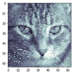
It's a cat alright.
Now, to apply the nonnegative matrix factorization! We use Scikit-Learn built-in coordinate descent optimization, and fitting the model is a matter of a few lines of code:
from sklearn.decomposition import NMF

nmf = NMF(n_components=50, max_iter=20)
nmf.fit(cats_data)

W = nmf.transform(cats_data)
H = nmf.components_
reconstr = np.dot(W, H)
The n_components parameter here is the reasonable amount of compression dimensions for our dataset. This number is usually difficult to determine - and based either on personal domain knowledge (i.e. "how many topics are possible in this dataset?"), or on parameter search using either grid search or an energy-based or elbow plot.
Note how we have now decomposed the original matrix (cats_data) into its W basis and H components. Hence we have 15747 vectors of length 50 - one per cat - which are a compressed representation of each cat; and 50 reduced features - or basis - each with dimension 4096 (64x64), which can be combined to create an infinite amount of cats.
print('the basis has dimension', H.shape, 'whereas the components have dimension', W.shape)

> the basis has dimension (50, 4096) whereas the components have dimension (15747, 50)
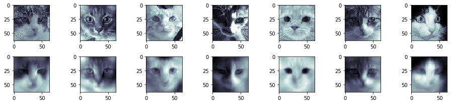
As mentioned, we evaluate the reconstruction ability of the model by simply taking the dot product of W and H.
This is how the original data (top row) and its reconstruction (bottom) compare:
compare_cats_plot(cats_data, reconstr, np.random.randint(0,len(cats_data),7))
And here are a few of the features that the model has been able to identify to distinguish between cats. We can see these features as activation vectors, which can be linearly combined to generate any cat from the dataset.
show_first_N_components(nmf, 5, 5, cmap='viridis')
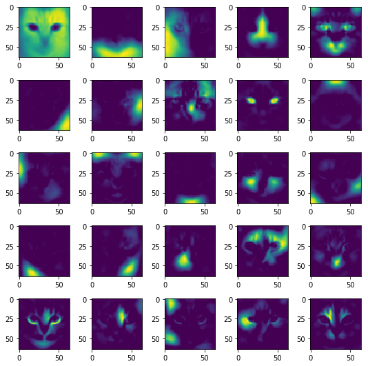
Clearly, the model has been able to identify a number of invariant spatial features (eyes, a nose, ears, eyes, ...), which make up a cat. This is basically a cat, reduced to its basic building blocks: NMF is useful to decompose complex data into its basic features (components) H, in order to understand exactly what is going on under a certain representation.
Even more interesting is the basis matrix H, which can be seen as a lower-dimensional representation of a cat's linearly combinable features. It would be really hard to classify or group cats based on their per-pixel view. However, the NMF model is able to distill the pixels down to H defining components, which are combined differently for each cat thanks to the basis H.
We can now apply clustering methods on the matrix H - but I'm already running out of time, so I'll simply write a simple search engine for cats:
def cosine_dist(vec, ind):
    dists = []
    for row in vec:
        dists.append(scipy.spatial.distance.cosine(row, vec[ind]))
    return pd.DataFrame(dists, columns=['cosine similarity'])


def get_similar_N(vec, ind, N):
    similar_rank = cosine_dist(vec, ind)
    return list(similar_rank.sort_values(by='cosine similarity').head(N+1).index[1:])


def get_dissimilar_N(vec, ind, N):
    similar_rank = cosine_dist(vec, ind)
    return list(similar_rank.sort_values(by='cosine similarity', ascending=False).head(N).index)


def plot_comparison_to(data, reconstructed, original, indexes, title=None):
    indexes = np.concatenate(([original], indexes))
    fig, ax = plt.subplots(2, len(indexes), figsize=(len(indexes)*2, len(indexes)/2))
    for i, ind in enumerate(indexes):
        ax[0, i].set_title("cat: "+str(ind))
        ax[0, i].imshow(get_square_image_from_array(data, ind), cmap='bone', interpolation='nearest')
        ax[1, i].imshow(get_square_image_from_array(reconstr, ind), cmap='bone', interpolation='nearest')
    ax[0, 0].set_title("search term:")
    plt.suptitle(title, y=1.05, size=20)
    plt.tight_layout()
    plt.plot()
Calculating the cosine similarity between a certain cat (the search term) and all other cats in the database allows us to find similar and different cats in the dataset.
The cosine similarity is a normed distance between two vectors, defined as:
\[ cosine(\pmb x, \pmb y) = \frac {\pmb x \cdot \pmb y}{||\pmb x|| \cdot ||\pmb y||} \]
A cosine similarity of 1 means we literally have two equally oriented vectors, whereas when cosine(x,y) is equal to zero, it means the two vectors are orthogonal.
cat_id = 4802
plot_comparison_to(cats_data,reconstr, cat_id, get_similar_N(W, cat_id, 8), 'most similar cats')
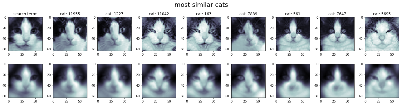
Sure enough, the compressed reconstruction (below) allows us to understand how the system sees the different cats (above) - and indeed, the system seems to be able to process queries based on visual elements (such as the 'parted black hair' left and right of this adorable cat's snout) rather than on per-pixel values.
plot_comparison_to(cats_data,reconstr, cat_id, get_dissimilar_N(W, cat_id, 8), 'most dissimilar cats')
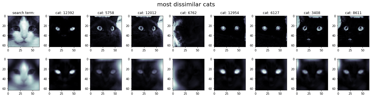
And obviously, we can also rank the cats by dissimilarity based on the search term, simply by flipping the cosine ranking. White cat with dark eyes usually returns a black cat with unsettling glowing peepers.
We can also feed these vector to downstream classifiers or unsupervised clustering methods. Feel free to build on top of the source code, as usual, in the 365ML github repo!