Today's dessert starts from a common problem: we have a series of observations in a cronological fashion. At a certain point in time the underlying process for the series might change: we want to detect this change, i.e. to train different models, before and after the switch point, while conserving uncertainty. How do we do that? One possible way is to use Bayesian statistics.
Recipe difficulty:
- Statistics: 🔥🔥🔥🔥 - using Bayesian models requires building the correct hierarchical models
- Technical: 🔥🔥 - nothing crazy, just some data manipulation
- Time required: 🕜 - around 2 hours from start to finish.
What it is
Bayesian statistics is a view on statistics where, instead of seeing the probability as a frequency of outcome, we look at it as a belief we have in the outcome. So if, say, a 50% probability of obtaining tails in a coin toss means we'll get tails 50 out of 100 tries in the frequentist view, in the Bayesian view it simply means that we have a 50% chance of obtaining that outcome on any coin throw.
This difference looks trivial, but it really isn't.
Why it matters
In the Bayesian framework, we do not observe an event multiple time and finally try to obtain unbiased estimates of its probability: rather, we approach each event with a prior belief of its probability: after the event completes we update our posterior belief in it by multiplying the prior with the observed outcome.
In other words, we do not simply look at the world as a blank slate: instead, we accept that we have prior information about the outcome of an event (i.e. we expect the coin to be either fair, or biased), and incorporate it in the experiment.
This means we can obtain more expressive estimates with less observations, and build complex hierarchical models which would be impossible in a purely frequentist estimation framework.
In this post, we're going to look at a series of airplane accidents, and try to understand whether the increased focus in regulations in the late sixties actually caused any noticeable change in the survival rate.
import pymc3 as pm
import pandas as pd
import numpy as np
import matplotlib.pyplot as plt

%matplotlib inline

planecrash = pd.read_csv('planecrash.csv',parse_dates=True)
planecrash = planecrash.groupby(planecrash['date'].dt.year)['fatalities_total','aboard_total'].sum().reset_index()
planecrash['fatal_percent'] = planecrash['fatalities_total']/planecrash['aboard_total']*100

years = planecrash["date"]
fatal = planecrash["fatal_percent"]
plt.rc('grid', linestyle="--", color='grey')
fig, ax = plt.subplots(1,1,figsize=(10,3), sharex=True)
ax.plot(planecrash['date'], planecrash['fatal_percent'], 'x', markersize=5, alpha=.8, label='fatality percent');
ax.plot(planecrash['date'], planecrash['fatal_percent'].rolling(20).mean(), alpha=.3, color='grey', label='rolling average');

ax.set_ylabel("fatalities percent")
ax.set_xticks(np.arange(1900,planecrash['date'].max()+1), minor=True)
ax.legend()
ax.xaxis.grid(which='minor', alpha=0.1)
ax.xaxis.grid(which='major', alpha=0.1)
plt.show()
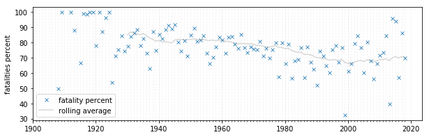
A visual analysis does not provide much insight on whether or when exactly something changed here. Luckily, we can use a Bayesian model for more critical analysis.
The peculiarity of Bayesian models is that you need to define your prior understanding of all variables involved.
Here we don't know where exactly the switch point would be: so we express the switchpoint variable as an Uniform distribution between the years range.
Similarly, we express the survival rates as Uniform distributions between 0 and 100.
Finally, we express the fatality rate as a Poisson distribution, which is quite expressive while only having a single parameter (the rate) for both scale and location.
Our model is therefore:
\[ \begin{align*} \text{switchpoint} & \approx \text{DiscreteUniform}(1915,2018) \newline
\text{fatal rate} & = \begin{cases}
\text{old rate}\approx\text{Uniform}(0,100) \newline
\text{new rate}\approx\text{Uniform}(0,100)
\end{cases} \newline
\text{fatal crashes} & \approx \text{Poisson}(\text{rate}) \end{align*} \]
with pm.Model() as plane_crash:

    switchpoint = pm.DiscreteUniform('switchpoint', years.min(), years.max())
    early_survival_rate = pm.Uniform('early_rate', 0, fatal.max())
    late_survival_rate = pm.Uniform('late_rate', 0, fatal.max())
    rate = pm.math.switch(switchpoint > years, early_survival_rate, late_survival_rate)
    fatal_crashes = pm.Poisson('disasters', mu=rate, observed=fatal)
with plane_crash:
    trace = pm.sample(5000, chains=2)

> Sampling 2 chains: 100%|████████████████████████████████████████████████████| 11000/11000 [00:05<00:00, 2032.97draws/s]
> The estimated number of effective samples is smaller than 200 for some parameters.
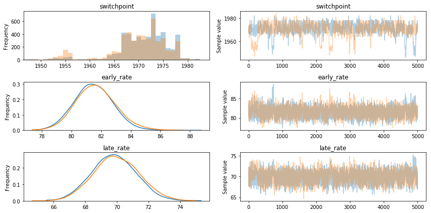
After sampling from the model, we obtain a Bayesian estimate of each parameter. Clearly:
- the most likely value for the switchpoint is around the turn of the decade between the 60s and the 70
- the early fatality rate is around 80%
- the later fatality rate is 10% lower, at around 70%
pm.traceplot(trace)
We can visualize what this means: the probability of the switchpoint is clearly concentrated around 1970, which is when the rate starts decreasing considerably and fans out.
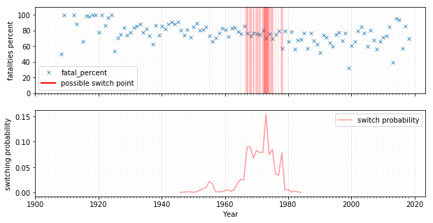
It indeed seems like the strong focus on aviation regulation in the industry in the late 60s pushed a change in the fatality average, lowering the stationary fatality rate by 10%. Good job!
More generally, it's hard to understate the usefulness and flexibility of Bayesian models: from finance, to commplex processes, to small data, to decision making; they are in my opinion much closer to how humans think than the standard frequentists frameworks that are taught in school, and are a valuable addition to any practitioner's toolset. Do try them out!