Today's recipe: let's take a look at a few common pitfalls of regular tabular ML and statistical models by understanding the difference between Causation and Correlation, and try it in action using the Causalinference package on Python.
Recipe difficulty
- Statistics: 🔥🔥 - the topic is hard, but this introduction will keep things as simple as possible
- Technical: 🔥 - easy peasy
- Time required: 🕜 - around 30 minutes max.
What it is
Whenever you .fit() a statistical model, either in Python or any other statistics language, you have to understand the gap between what you want to measure and what you're actually measuring.
For instance, let's say we're developing a model for a company selling ice-cream in supermarkets. We measure a lot of datapoints about customers, and discover an interesting relationship: it seems that customers carrying umbrellas tend not to buy our ice-cream, and buy hot chocolate instead, whereas customers wearing sunglasses tend to buy our product in large quantities.
This is correlation - what you actually measured in the real world. Obviously it's not what you wanted to measure: what you (or your boss) wanted was a predictive model for targeting potential ice-cream customers. And that's where the pitfall lies.
We can safely conclude, in this case, that there is no causal relationship between umbrellas, sunglasses and ice-cream. The relationship is rather weather -> attire and weather -> ice-cream. If you were to run to your boss with an advertising pitch to send everyone in town a free pair of sunglasses in order to drive ice-cream sales, you'd be regarded as crazy and sent back to your computer with nothing more than a good laugh.
Why is it useful?
Your boss does not laugh in the real world: instead, you get promoted. Indeed, virtually any machine learning model deployed in a production scenario nowadays is a correlation model, not a causation model. If you work in the sector, and chuckled at the ice-cream example, stop right now: for most of the models you've developed so far suffer from this exact same problem.
In many cases, a correlation model is perfectly fine. But when the data size is limited and the amount of counterfactuals very high, basing any decision on a statistical model with little thinking can and will lead to catastrophic outcomes.
Let's take for instance this dataset about student outcomes in Spain. A very common problem in economics and social sciences is the allocation of short-term resources (such as funding and man-hours) to long-term projects (such as inclusion programs, incentives and citizen assistance) in the hope of obtaining a long-term return (economic boost, highly-educated workers, increase in productivity) that is larger than the invested resources.
In this particular case, this mouthful basically translates to the following research question: does it make sense to spend money paying for kids' assistance in order to make them study more?
df_data.head()| sex | romantic | health | goout | famrel | absences | Dalc | Walc | famsup | studytime | |
|---|---|---|---|---|---|---|---|---|---|---|
| 0 | 1 | 0 | 3 | 4 | 4 | 6 | 1 | 1 | 0 | 2 |
| 1 | 1 | 0 | 3 | 3 | 5 | 4 | 1 | 1 | 1 | 2 |
| 2 | 1 | 0 | 3 | 2 | 4 | 10 | 2 | 3 | 0 | 2 |
| 3 | 1 | 1 | 5 | 2 | 3 | 2 | 1 | 1 | 1 | 3 |
| 4 | 1 | 0 | 5 | 2 | 4 | 4 | 1 | 2 | 1 | 2 |
In an ideal world, we'd just take exactly half the kids, assign them to the assistance program, take the other half and give them no additional assistance at all; then compare the difference in study hours between the two cohorts pre- and post-treatment. This is called a randomized controlled trial and it's basically the single most important tool in modern science.
For our particular dataset, we'd be interested in determining the direction and significance of:
\[ E[Y_{\text{hours studied}}|D_{\text{assistance}}] - E[Y_{\text{hours studied}}|D_{\text{no assistance}}] \]
But in the real world, it's often unethical or unfeasible to do so - hence kids were not assigned to either group (the treatment group - that is, the one with assistance - or the control group).
Very often, this type of effects are incredibly difficult to spot - and even more difficult to correct. We are therefore able to identify correlation between co-variates and our target variable, but the two key assumptions of causality are violated.
What are these two assumptions?
- Overlap: $ 0 < P(D_{\text{assistance}} | X_i = x) < 1 \text{for any }x ∈ X $
In layman's term, this means that the two cohorts have underlying similarity across all dimensions. For instance, if we only had one explanatory co-variate:
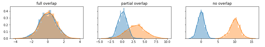
Having no overlap means the groups (treatment and control) would already be intrinsically different - and any conclusion we might find about the effectiveness of the treatment are probably moot.
- Unconfoundness: $ Y\perp D|X_i = x \text{for any }x ∈ X $
This means the target variable Y is completely independent of the treatment conditioned on the co-variate set X. Concretely, this means we have to even out the effect of co-variates X on the treatment outcome Y by correcting for them in the causal model. That is, the treatment D can only affect Y without conditioning on the co-variates; when there is conditioning, the effect of treatment of outcome should be random.
In layman's terms, the co-variates X cannot affect the choice of receiving treatment or not.
In our specific case, we already know the second assumption is violated: we know the data is not a randomized trial, and therefore the outcome Y will be affected by the co-variates X's effect on D.
We can start by testing our first assumption using the fantastic causalinference python package:
from causalinference import CausalModel

Y_observed = df['studytime']
D_treat = df['famsup']
covariates = ['sex','romantic','health','goout','famrel','absences','Dalc','Walc']
K_covariates = df[covariates]

cm = CausalModel(Y_observed, D_treat, K_covariates.values)
What we are doing here is creating a CausalModel object, which requires three sets of variables:
- Y, the observed outcome. It's what we want to measure.
- D, the treatment. It's what we do to causally affect the outcome. In do-calculus terms, $ P(Y|\text{do}(D)) $
- X, the set of co-variates or individual charachteristics for each unit, which are potentially affecting either Y or D
In this case we know, given how the dataset was made, that the co-variates X are affecting D. If we have some overlap, however, we can correct for this problem.
To verify overlap between groups in a multivariate context, we use the normalized score:
\[ \text{normalized score} = \frac{\overline{X_{\text{treat}}}-\overline{X_{\text{control}}}}{\sqrt{(S2_{\text{treat}}+S2_{\text{control}})/2}} \]
There's no hard rules for the normalized score - in general, if its absolute value is above 0.5/1 we'd have some doubts about having sufficient coverage for our causal correction. In this case, however, the normalized difference is well between ± 0.5 for all co-variates:
print(cm.summary_stats)Summary Statistics
Controls (N_c=125) Treated (N_t=224)
Variable Mean S.d. Mean S.d. Raw-diff
--------------------------------------------------------------------------------
Y 1.880 0.829 2.165 0.849 0.285
Controls (N_c=125) Treated (N_t=224)
Variable Mean S.d. Mean S.d. Nor-diff
--------------------------------------------------------------------------------
X0 0.416 0.495 0.585 0.494 0.341
X1 0.328 0.471 0.321 0.468 -0.014
X2 3.512 1.418 3.612 1.365 0.072
X3 3.192 1.141 3.067 1.112 -0.111
X4 4.016 0.871 3.929 0.875 -0.100
X5 5.944 9.049 5.978 7.941 0.004
X6 1.488 0.858 1.420 0.859 -0.080
X7 2.416 1.381 2.174 1.260 -0.183
The overlap assumption is covered, and we can now move on to correct for the unconfoundness assumption. This is where a naive ML model would lead us to the wrong confusion. Let's see one of these naive models: a regular linear regression.
import statsmodels.api as sm

results = sm.OLS(Y_observed, sm.add_constant(x)).fit()
print(results.summary())
OLS Regression Results
==============================================================================
Dep. Variable: y R-squared: 0.137
Model: OLS Adj. R-squared: 0.114
Method: Least Squares F-statistic: 5.974
Date: Sun, 10 Mar 2019 Prob (F-statistic): 9.02e-08
Time: 16:05:12 Log-Likelihood: -413.12
No. Observations: 349 AIC: 846.2
Df Residuals: 339 BIC: 884.8
Df Model: 9
Covariance Type: nonrobust
==============================================================================
coef std err t P>|t| [0.025 0.975]
------------------------------------------------------------------------------
const 1.9169 0.274 6.993 0.000 1.378 2.456
sex 0.3952 0.092 4.276 0.000 0.213 0.577
romantic 0.1305 0.094 1.386 0.167 -0.055 0.316
health -0.0295 0.032 -0.926 0.355 -0.092 0.033
goout 0.0205 0.043 0.476 0.634 -0.064 0.105
famrel 0.0234 0.051 0.458 0.647 -0.077 0.124
absences -0.0076 0.005 -1.431 0.153 -0.018 0.003
Dalc 0.0035 0.067 0.052 0.958 -0.128 0.135
Walc -0.1076 0.048 -2.245 0.025 -0.202 -0.013
famsup 0.2014 0.091 2.206 0.028 0.022 0.381
It seems indeed like having family support has a positive impact on the study time. The effect is significantly positive, and we'd accept the null hypothesis at the 5% level: giving family support seems to positively affect the student's engagement.
Note that we can do the same using Causalinference alone:
cm.est_via_ols(adj=1)
print(cm.estimates['ols'])
Treatment Effect Estimates: OLS
Est. S.e. z P>|z| [95% Conf. int.]
--------------------------------------------------------------------------------
ATE 0.201 0.088 2.289 0.022 0.029 0.374
Same effect, same p-value as expected.
But is this actually correct?
As demonstrated by Rosenbaum and Ruben in 1983, we can actually see if any particular covariate influences the distribution to the treatment or control groups for participants by calculating propensity scores.
A propensity score is simply the probability of being assigned to a specific group (treatment or control) D, given the vector of covariates X. Formally:
\[ \text{propensity score} = P(D_\text{treatment}|X)
\]
The concept is surprisingly simple - this is really just a logistic regression - indeed, we can calculate the results using alogistic regression model:
results = sm.Logit(D_treat, sm.add_constant(K_covariates)).fit()
or, more aptly, using Causalinference. The results are exactly the same:
cm.est_propensity()
print(cm.propensity)
Estimated Parameters of Propensity Score
Coef. S.e. z P>|z| [95% Conf. int.]
--------------------------------------------------------------------------------
Intercept 0.650 0.711 0.914 0.361 -0.744 2.044
X0 0.685 0.242 2.831 0.005 0.211 1.160
X1 -0.122 0.250 -0.491 0.624 -0.612 0.367
X2 0.111 0.084 1.320 0.187 -0.054 0.275
X3 -0.033 0.115 -0.291 0.771 -0.258 0.191
X4 -0.131 0.137 -0.963 0.336 -0.399 0.136
X5 -0.000 0.014 -0.004 0.996 -0.028 0.028
X6 0.143 0.174 0.823 0.411 -0.197 0.483
X7 -0.150 0.125 -1.199 0.230 -0.396 0.095
What this tells us is that variable X0 - sex - is driving assignment to the control/treatment group in a significant manner. Indeed, we can use a simple exponential link to calculate the probability of being assigned to the treatment group for each sample in our dataset. Let's take for instance the very first pupil in the dataset:
| sex | romantic | health | goout | famrel | absences | Dalc | Walc | famsup | |
|---|---|---|---|---|---|---|---|---|---|
| 0 | 1 | 0 | 3 | 4 | 4 | 6 | 1 | 1 | 0 |
The probability of this pupil to belong to the treatment group is 73.11% (this is obviously a chance estimation: this pupil was actually assigned to the control group in the observed state of our world).
def estimate_treat(cm, variables):
    coefs = cm.propensity['coef']
    return 1/(1+np.exp(-(coefs[0]+np.dot(variables, coefs[1:])))) # logit link

estimate_treat(cm, [1,0,3,4,4,6,1,1])

> 0.7311
We can now use these propensity score to match together similar people from the cohort group based on their score, which in turn is based on their individual features X. The intuition is simple: we look for pupils which are similar with regard to the co-variates X which, as we recall, we suspected of influencing their assignment to the treatment and control groups. We then calculate the difference between pairs (or triplets, quadruples, ...):
\[ \mathrm{E}[Y_{\text{i, treated}}-Y_{\text{i, control}}|X] \text{ for each } i_{\text{th}} \text{ pair}\]
By averaging this effect across all pairs (which are sampled with replacement) we obtain the final treatment effect.
cm.est_via_matching(matches = 1, bias_adj=True)
print(cm.estimates['matching'])
Treatment Effect Estimates: Matching
Est. S.e. z P>|z| [95% Conf. int.]
--------------------------------------------------------------------------------
ATE 0.180 0.151 1.195 0.232 -0.115 0.476
Sure enough, the Average Treatment Effect is still positive, but actually insignificant this time around. We cannot significantly reject the null-hypothesis "the school assistance program has no impact on the actual hours studied" whenever we use the matching estimator.
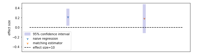
Hence, we have been able to disprove the refutation of our null-hypothesis. If we were deploying this model, we'd probably have to find more co-variates or focus on different types of treatment (or actually run a fully randomized trial), since our naive ML regression is actually wrong.
This whole disproving mechanism is one of the cores of causal inference - a field that significantly overlap with my major interest (Bayesian statistics), is seeing a significant increase in attention and research in the last few years as machine learning becomes more and more prominent. A field, in short, which i strongly recommend you look into, lest you find yourself recommending sunglasses instead of ice-cream advertisements on your daily job.